Processes on the Sun can accelerate protons to relativistic energies, producing Solar Proton Events (SPE), also known as Solar Energetic Particle (SEP) events. Arguments continue as to whether the acceleration is driven by the X-ray flare release process or in solar wind shock fronts during coronal mass ejections [Krucker and Lin, 2000; Cane et al., 2003]. The high-energy component of this proton population is at relativistic levels such that they can reach the Earth within minutes of solar X-rays produced during any solar flares which may be associated with the acceleration. Satellite data show that the protons involved have an energy range spanning 1 to 500 MeV, occur relatively infrequently, and show high variability in their intensity and duration [Shea and Smart, 1990]. For large events the duration is typically several days, with risetimes of ~1 hour, and a slow decay to normal flux values thereafter [Reeves et al., 1992].
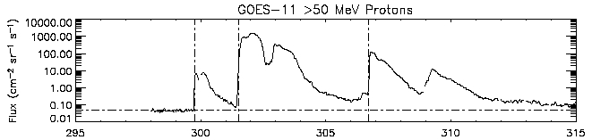
Figure 1. >50 MeV proton fluxes measured by the GOES-11 satellite during a series of solar proton events during the period 22 October to 10 November 2003. (After Clilverd et al. [2006]).
The most energetic SPE population deposits its energy at altitudes as low as 20-30 km, producing ionization and changing the local atmospheric chemistry. SPE particles generally lie at energies below which nuclear interaction-losses will be significant, such that ionization-producing atmospheric interactions are the dominant energy loss. Figure 2 shows calculated atmospheric ionization rates determined from the GOES-11 proton fluxes for the period 26 Oct-7 Nov 2003 using the Sodankylä Ion Chemistry model. Particle precipitation results in enhancement of odd nitrogen (NOx) and odd hydrogen (HOx). NOx and HOx play a key role in the ozone balance of the middle atmosphere because they destroy odd oxygen through catalytic reactions [e.g., Brasseur and Solomon, 1986, pp. 291-299].SPE-produced ionization changes tend to peak at ~70 km altitude [Clilverd et al., 2005a], leading to local perturbations in ozone levels [Verronen et al., 2005]. Figure 3 shows odd oxygen changes, which includes the loss of ozone calculated by the Sodankylä Ion Chemistry model during the Oct-Nov 2003 SPE period. While the ozone destruction at such high altitudes is generally not important to the total ozone population, under some conditions NOx can be long-lived, particularly during polar winter at high latitudes. In this situation vertical transport can drive the NOx down towards the large ozone populations in the stratosphere, leading to large long-lived ozone depletions [e.g., Reid et al., 1991]. Changes in NOx and O3 consistent with SPE-driven modifications have been observed [Seppälä et al., 2004, Verronen et al., 2005], and large depletion in ozone during the Arctic winter have been associated with a series of large SPEs over the preceding months [Randall et al., 2005].
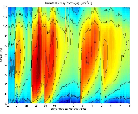
Figure 2. Ionization rates in the atmosphere calculated using SIC based on GOES-11 proton flux measurements (26 Oct -7 Nov 2003). (After Verronen et al. [2005]).
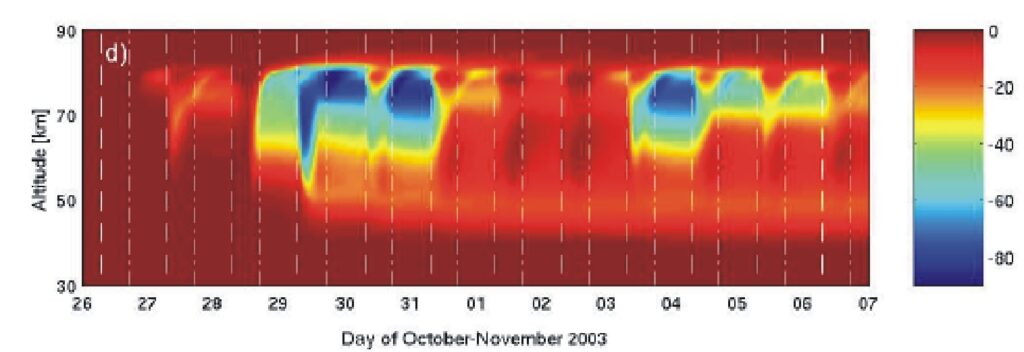
Figure 3. Middle atmospheric response to the proton events (SIC modelling results) in Oct-Nov 2003. This panel shows the relative change in Ox (which includes O3) due to SPE-forced chemical changes. (After Verronen et al. [2005]).
SPE particles cannot, however, access the entire global atmosphere as they are partially guided by the geomagnetic field. The first description of cosmic rays in the Earth’s magnetic field [Störmer, 1930] demonstrated the geomagnetic cutoff rigidity, the minimum rigidity a particle must possess to penetrate to a given geomagnetic latitude, where the rigidity of a particle is defined as the momentum per unit charge. Therefore, every geomagnetic position has a corresponding cutoff rigidity. Higher rigidities are required to reach lower geomagnetic latitudes, and thus all particles with rigidities larger than the minimum can penetrate to that latitude (and all higher latitudes). In general the geomagnetic cutoff rigidity of a particle is also a function of its direction of arrival. While this effect was initially modeled with a static dipole field, the geomagnetic cutoff rigidity is a much more dynamic quantity depending on the Earth’s internal and external magnetic fields. As such the geomagnetic cutoff varies spatially and with time, on timescales of both the internal (years) [Smart and Shea, 2003b] and the external field (minutes-hours) [Kress et al., 2004].
Experimental measurements of geomagnetic cutoff rigidities have generally been based on satellite observations, while theoretical calculations have primarily focused on tracing particles through models of the Earth’s field producing grids of estimated cutoff rigidities distributed over the Earth at a given altitude [e.g., Smart and Shea, 1985]. Comparisons between satellite-derived rigidity cutoffs and those determined by particle tracing studies generally show the measured cutoff latitudes are several degrees lower than the theoretical values [e.g., Fanselow and Stone, 1972]. However, new calculations undertaken using improved geomagnetic field models have resulted in lower rigidity-determined latitude cutoffs than earlier particle tracing studies [e.g., Smart et al., 2003a], improving this comparison.
Generally, the satellite-derived cutoff rigidities have neglected the dynamic nature of the magnetic field, by considering the average magnetic field configuration present over a long time period [e.g., Ogliore et al., 2001] or for a relatively fixed disturbance level (i.e., a fixed Kp value) during a short time period [e.g., Dyer et al., 2003]. Due to the low-orbital altitudes of most of the satellites involved, few experimental studies have derived cutoffs during the most disturbed conditions during geomagnetic storms. One example, however, is the injection and formation of a new proton population in the inner radiation belt triggered by a large solar wind density enhancement compressing the cutoff rigidities for the 23-24 November 2001 storm [Kress et al., 2004]; here the dynamic modeling of the cutoff values lead to additional understanding of SPE particle access to the inner magnetosphere.
As noted above, the impact of SPE particles upon the upper atmosphere leads to significant additional ionization, which can be detected through ground-based observations. The ionospheric effects of SPEs were first identified through the large absorption increases in VHF communications during the 23 February 1956 event [Bailey, 1957]. Long-range remote sensing of SPE-produced ionospheric modifications has been undertaken by examining the phase and amplitude changes of LF and VLF transmissions propagating beneath the ionosphere [e.g., Westerlund et al., 1969]. Recent studies have contrasted calculated electron density profiles output from a SPE-driven atmospheric chemistry model with radio propagation observations, particularly for the 4-10 November 2001 [Clilverd et al., 2005a] and October/November 2003 storms [Verronen et al., 2005; Clilverd et al., 2005b]. An example of subionospheric amplitude changes received during the October/November 2003 storms is shown in Figure 4. These studies have shown that our understanding of VLF propagation influenced by SPEs is high, such that VLF observations might be used to predict changes in the ionospheric D-region electron density profiles during other particle precipitation events. However, observations of subionospheric propagation of long wavelength electromagnetic waves are not well-suited for determining geomagnetic cutoff rigidities. While studies have shown these techniques are well-suited for testing ionospheric modification profiles [e.g., Clilverd et al., 2005a], even short paths partially affected by SPE ionization are dominated by the altered ionosphere. During the October/November 2003 SPEs, the path from a transmitter in Iceland to a receiver in Erd, Budapest was modeled by applying a SPE-modified ionosphere to the first 500 km of the ~3000 km path [Clilverd et al., 2005b]. The propagation modeling showed remarkably good agreement with the SPE-influenced data, despite the small percentage of the path which will have been affected by the SPE precipitation.
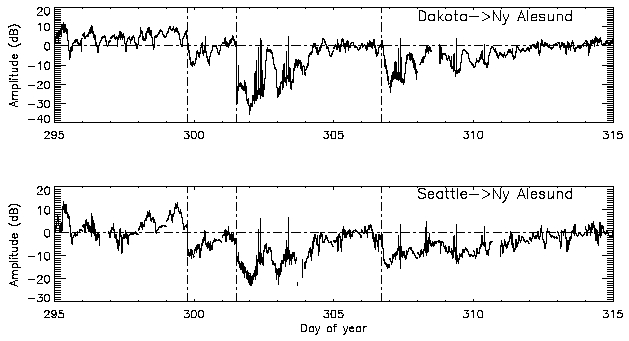
Figure 4. Amplitude change of subionospheric VLF transmissions received by the AARDDVARK at Ny Alesund, during 20 days in October/November 2003. The change is relative to the respective quiet day curves of signals from that transmitter at this receiver. The times of the onset of solar proton events are indicated by the vertical dashed lines(After Clilverd et al. [2006]).
In contrast, riometers (relative ionospheric opacity meter), which measure the absorption of cosmic radio noise at a given frequency (usually 20-40 MHz) provide essentially overhead measurements of ionization levels, and are well suited for examining geomagnetic cutoffs. This is particularly true for imaging riometer systems (IRIS) where large receiver arrays provide an image of the ionospheric absorption levels above the instrument [Detrick and Rosenberg, 1990]. It has been shown that there is an empirical relationship between the square root of the integral proton flux (>10 MeV) and cosmic noise absorption (CNA) in daytime, at least when geomagnetic cutoff effects do not limit the fluxes [Kavanagh et al., 2004]. The same study concluded that variations in the spectral hardness of the SPE proton flux and atmospheric collision frequencies do not cause significant departures from the linear relationships observed.
SPEs are major, though infrequent, space weather phenomena that can produce hazardous effects in the near-Earth space environment. The occurrence of SPE during solar minimum years is very low, while in active Sun years, especially during the falling and rising phases of the solar cycle, SPEs may average one per month. The impacts of SPEs include ‘upsets’ experienced by Earth-orbiting satellites, increased radiation exposure levels for humans onboard spacecraft and high-altitude aircraft, ozone depletions and disruption to HF/VHF communications in mid- and high-latitude regions. A detailed understanding of all these impacts depends upon knowledge of the dynamic rigidity cutoffs imposed by the changing total magnetic field.
References
References for the papers cited in this background material piece are listed together on another webpage.
[Note: This background material is drawn from the introduction section of our paper:
Rodger, C. J., M. A. Clilverd, P. T. Verronen, Th. Ulich, M. J. Jarvis, and E. Turunen, Dynamic geomagnetic rigidity cutoff variations during a solar proton event, J. Geophys. Res., 111, A04222, doi:10.1029/2005JA011395, 2006.]